Homework 10
Isabelle Smith
2025-04-09
Libraries
##install.packages("tidytuesdayR")
library(tidytuesdayR)
library(tidyverse)
library(ggridges) # ridge plots
library(ggbeeswarm) # beeswarm plots
library(GGally) # parallel coordinates plots
library(ggpie) # pie charts
library(ggmosaic) # mosaic plots
library(scatterpie) # scatter pies on map
library(waffle) # for waffle plots
library(DescTools) # for converting table to long
library(treemap) # for tree maps
Work
Use your newly-developed ggplot chops to create some
nice graphs from a dataset from the TidyTuesday
Dataset project. You can make any combination of four plots from the
list below:
- Beeswarm Plot
- Ridgeline Plot
- Pie Charts
- Mosaic Plot
- Scatter Pie Plot
- Waffle Plot
- Tree Map
- 2-D Density Plot
- Dendrogram
0. Data
I chose the Palm Trees dataset.
tuesdata <- tidytuesdayR::tt_load(2025, week = 11)
palmtrees0 <- tuesdata$palmtrees


palmtrees <- palmtrees0 |>
  dplyr::select(spec_name, acc_genus, palm_tribe, palm_subfamily,
         climbing, erect, max_stem_height_m, max_stem_dia_cm,
         average_fruit_length_cm, average_fruit_width_cm,
         fruit_size_categorical, fruit_shape, conspicuousness) |>
  drop_na() |>
  rename(fruit_conspic=conspicuousness)
palmtrees |>
dplyr::select(where(is.numeric)) |>
summary()## max_stem_height_m max_stem_dia_cm average_fruit_length_cm
## Min. : 0.00 Min. : 0.00 Min. : 0.400
## 1st Qu.: 3.00 1st Qu.: 2.50 1st Qu.: 1.100
## Median : 8.00 Median : 6.00 Median : 1.550
## Mean : 12.37 Mean : 13.61 Mean : 2.189
## 3rd Qu.: 18.00 3rd Qu.: 20.00 3rd Qu.: 2.500
## Max. :170.00 Max. :175.00 Max. :30.000
## average_fruit_width_cm
## Min. : 0.215
## 1st Qu.: 0.800
## Median : 1.150
## Mean : 1.623
## 3rd Qu.: 1.800
## Max. :20.000palmtrees |>
dplyr::select(!where(is.numeric)) |>
mutate(across(everything(), function(x) length(unique(x)))) |>
filter(row_number()==1) |>
as.data.frame() |>
`rownames<-`("n_unique") |>
t()## n_unique
## spec_name 1111
## acc_genus 163
## palm_tribe 27
## palm_subfamily 5
## climbing 3
## erect 3
## fruit_size_categorical 2
## fruit_shape 7
## fruit_conspic 2d3_colors <- ggsci::pal_d3("category10")(10)
1. Waffle Plot
shape_table <- as.data.frame(table(shape=palmtrees$fruit_shape))

shape_colors <- c(d3_colors[1],
                  d3_colors[2],
                  d3_colors[10],
                  "darkolivegreen3", #d3_colors[9],
                  d3_colors[5],
                  d3_colors[3],
                  d3_colors[4])


ggplot(data=shape_table) +

  aes(fill = shape, values = Freq) +

  waffle::geom_waffle(n_rows = 25, size = 0.33, colour = "white") +

  scale_fill_manual(values=shape_colors) +

  coord_equal() +

  theme_void() +

  labs(title="Fruit Shapes of Palm Trees",
       fill=NULL) +

  theme(plot.title=element_text(hjust=0.5, vjust=4),
        plot.subtitle=element_text(hjust=0.5, vjust=4),
        plot.caption=element_text(vjust=-7),
        axis.title.x=element_text(vjust=-4),
        axis.title.y=element_text(vjust=5),
        plot.margin=margin(1, 1, 1, 1, "cm"),
        legend.position="top",
        legend.key.size = unit(0.02, 'npc')) +

  guides(fill = guide_legend(nrow = 1))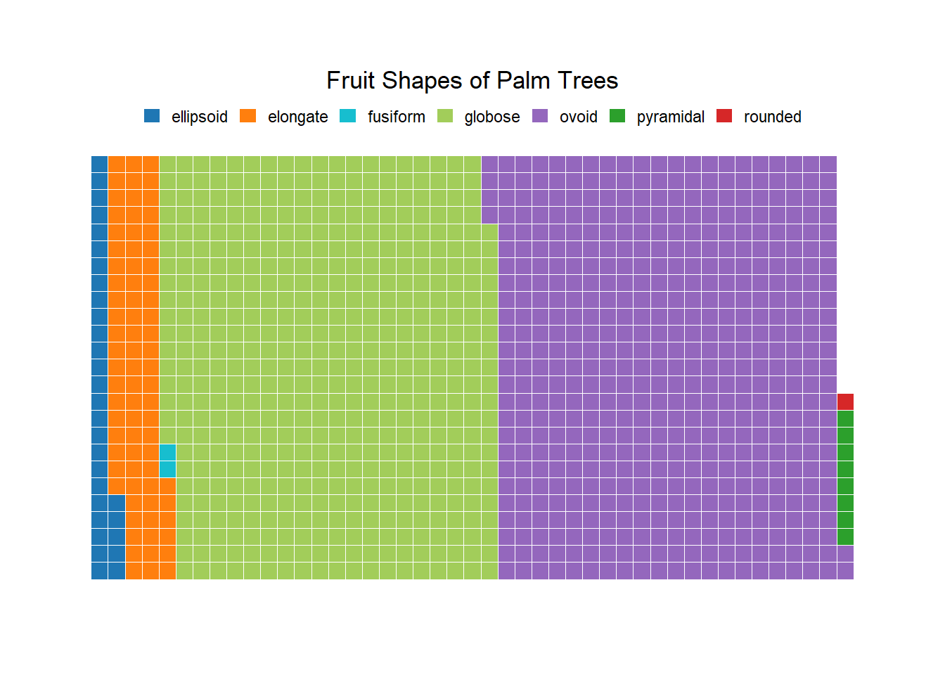
2. Tree Map
EC_table <- as.data.frame(table(Erect=palmtrees$erect,Climbing=palmtrees$climbing))


## increasing low counts for visualization purposes
EC_table_e <- EC_table |> mutate(Freq = case_when(Freq==0 ~ 0,
                                                 Freq < 10 ~ Freq + 20,
                                                 TRUE ~ Freq))

treemap(dtf=EC_table_e,
        index=c("Erect","Climbing"),
        vSize="Freq",
        type="index",
        title="Palm Tree Characteristics",
        fontsize.labels = c(11, 7),
        orce.print.labels= T,
        fontcolor.labels = c("black", "white"),
        align.labels = list(c("left", "top"), c("right", "bottom")),
        aspRatio=1.75)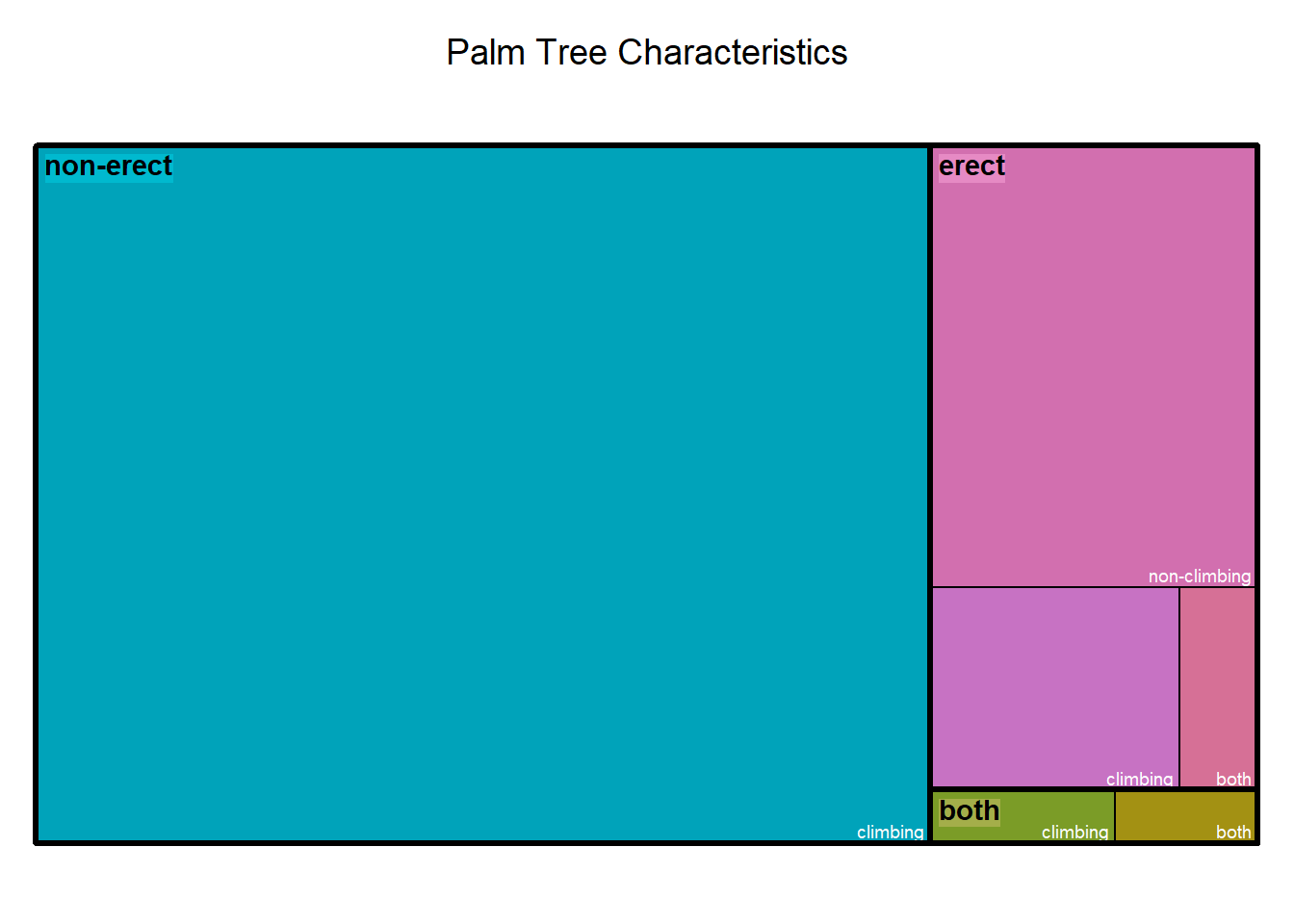
3. Scatterpie
fruit_df_f <- palmtrees |>

  ## filtering size for visualization purposes
  filter(average_fruit_length_cm<10, average_fruit_width_cm<10) |>

  mutate(length_c = round(average_fruit_length_cm),
         width_c = round(average_fruit_width_cm),
         conspicuous = case_when(fruit_conspic=="conspicuous" ~ 1,
                                 fruit_conspic=="cryptic" ~ 0),
         cryptic = case_when(fruit_conspic=="cryptic" ~ 1,
                             fruit_conspic=="conspicuous" ~ 0)) |>

  group_by(length_c,width_c) |>

  summarize(n = n(),
            conspicuous=sum(conspicuous),
            cryptic=sum(cryptic),
            .groups="drop")


ggplot(data=fruit_df_f) +
  scatterpie::geom_scatterpie(
    aes(x=width_c, y=length_c),
    pie_scale=2,
    cols=c("conspicuous", "cryptic")) +
   coord_equal() +
  scale_fill_manual(values=c("coral","turquoise")) +
  labs(title="Distribution of Palm Tree Fruit",
       x="Average Width",
       y="Average Length",
       fill="Color Type") +

  theme(plot.title=element_text(hjust=0.5, vjust=4),
        plot.subtitle=element_text(hjust=0.5, vjust=4),
        plot.caption=element_text(vjust=-7),
        axis.title.x=element_text(vjust=-4),
        axis.title.y=element_text(vjust=5),
        plot.margin=margin(1, 1, 1, 1, "cm"),
        legend.position="right")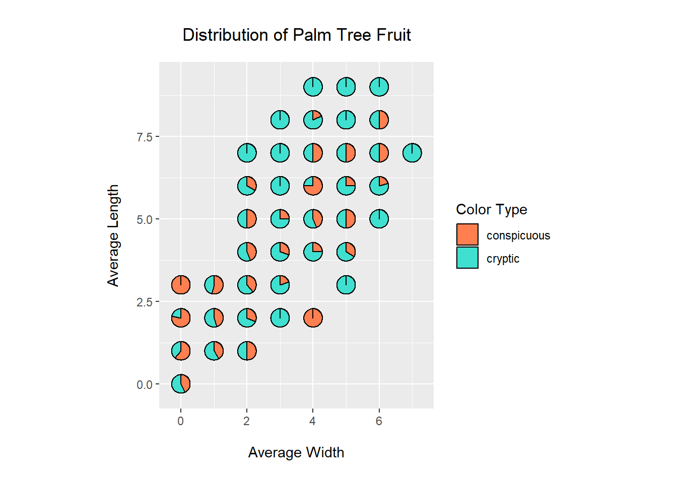
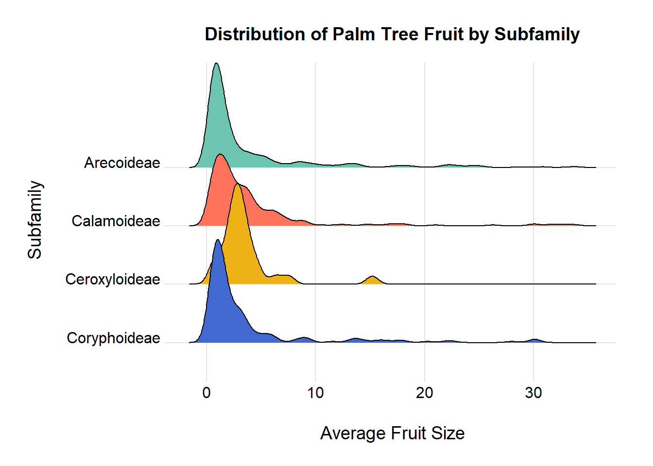
4.
size_df <- palmtrees |>

  mutate(average_fruit_size = average_fruit_length_cm * average_fruit_width_cm,

         ## reversing order to be alphabetical in visualization
         palm_subfamily_r = fct_rev(palm_subfamily))


size_df_f <- size_df |>

  ## filtering size for visualization purposes
  filter(average_fruit_size < 35)


ggplot(data=size_df_f) +

  aes(x=average_fruit_size,y=palm_subfamily_r,fill=palm_subfamily_r) +

  ggridges::geom_density_ridges() +

  ggridges::theme_ridges() +

  ggsci::scale_fill_observable() +

  labs(title="Distribution of Palm Tree Fruit by Subfamily",
       x="Average Fruit Size",
       y="Subfamily") +

  theme(plot.title=element_text(hjust=0.5, vjust=4),
        plot.subtitle=element_text(hjust=0.5, vjust=4),
        plot.caption=element_text(vjust=-7),
        axis.title.x=element_text(hjust=0.5, vjust=-4),
        axis.title.y=element_text(hjust=0.5, vjust=5),
        plot.margin=margin(1, 1, 1, 1, "cm"),
        legend.position="none")
## Picking joint bandwidth of 0.564